Overview of the model work flow

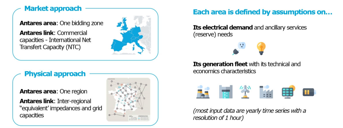
The power system is represented with a graph involving up to a few hundreds of country-sized or region-sized nodes, tied together by edges whose characteristics summarize those of the underlying power grid. Each node includes a description of its electrical demand, its reserve needs and its generation fleet, this last being composed of thermal units, hydro units (run-of-river units and seasonal reservoirs), intermittent renewable generation, pumping stations and storages.
Power flows are either ruled by Net Transfer Capacities (NTC) or by a conventional DC approximation with data in form of PTDF or impedances. In both cases, additional binding constraints between flows can represent specific market rules (such as flow-based market coupling) and/or physical components (such as phase-shifting devices, DC lines).
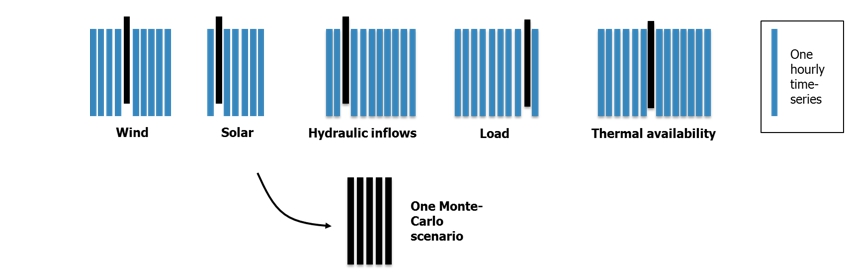
Five inputs can be described as random variables in Antares: Availability of thermal power plants, load, wind power generation, solar generation and hydraulic inflows.
They are represented in the software with several time-series, each one being a possible realisation of the variable for the studied future horizon. The probabilistic Monte-Carlo method embedded in Antares consists in simulating the response of the power system to many situations that it could face, for instance (see below) many maintenance schedules and outages time-series of the generation units.
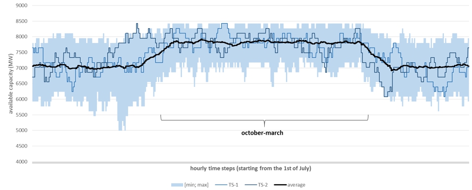
Availability time series of a thermal cluster of 8.4 GW. Minimum, maximum, average values over 60 time-series, and two specific samples. The time-series have been generated with Antares (see also time series analysis and generation).
Time series of the random variables can be either extracted from ad hoc data banks or generated within the tool by built-in specialized modules: the time series analyser and the time-series generator.
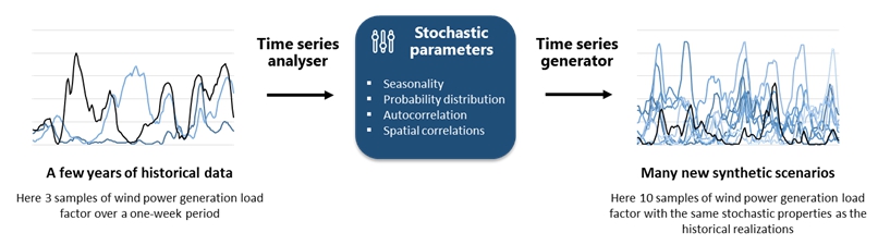
Working principle of the time series analyser and time series generator
The time series analyser learns from external data (typically from historical data) intrinsic characteristics of their stochastic behaviour :
- their seasonalities - e.g. daily and yearly climatic cycles impacting PV generation
- their probability distribution functions,
- their autocorrelation functions
- and their spatial correlations - e.g. correlations between wind regimes of adjacent areas.
The time series generator randomly draws new samples of stochastic processes based on given values of the aforementioned characteristics. The generated set respects the same global characteristics as the learning sample, but each generated time series has its own specificities, for instance a low wind generation which occur during a day when the wind was always high in the learning sample.
The combined use of these two modules allows to enrich the Monte-Carlo approach with new situations that did not occur in past records but could possibly happen in the future. These two modules are independent and can also be run separately. For instance, the time-series generator can be supplied with stochastic parameters obtained with another source than the time series analyser.
Once all the random variables have been set, using external data or time series generated within Antares, Monte-Carlo scenarios can be defined by combining the different contingencies.
Antares contains a Monte-Carlo scenario builder which allows to define a picking strategy for each Monte-Carlo scenario. The selection can be:
- prespecified, mentionning which time-series to use for each Monte-Carlo scenario,
- random (in that case, some rules can be defined to keep the consistency of correlations between variables and/or areas),
- or a combination of both, with different strategies depending on the variables and areas.
For each of the defined Monte-Carlo scenario, Antares then simulates the operation of the system throughout the year
For each Monte-Carlo scenario, Antares optimizes the unit-commitment and dispatch so as to meet the demand at the lowest cost. Each year is seen as a succession of weekly optimization sub-problems whose objective is the minimization of the electricity supply costs. All of these problems are defined at the spatial scale of the whole interconnected system. The kernel of the software is a linear solver developed by RTE which computes operating set-points for the whole system (optimal weekly unit-commitment, hydro-thermal scheduling and interconnection flows with an hourly resolution).
So as to deal conveniently with some difficult aspects of hydro-thermal optimal unit-commitment and dispatch (presence of both integer and real variables), simulation settings allow different formulations of the optimization problem with several trade-offs between computation time and accuracy. The most exhaustive simulation mode includes explicitly in the optimization problem the unit-commitment variables and the constraints and costs related to the flexibility of the generation units (minimum stable power, minimum up and down durations, start-up costs, no-load heat costs), while fastest modes solve a simplified (yet accurate enough for most uses) version of this problem within very short times.
The task of the immediately upper level is to assess and provide to the inner optimization kernel weekly hydraulic energy volumes to generate from the different reservoirs of the system, for each week of the current Monte-Carlo year. It is indeed mandatory to materialize the coupling effect that the medium and long term management of hydraulic resources introduces between the successive short term weekly optimization sub-problems. To perform its task, this module makes use of general assumptions describing the reservoir capacities and their management strategies, as well as rainfall scenarios for the current year.
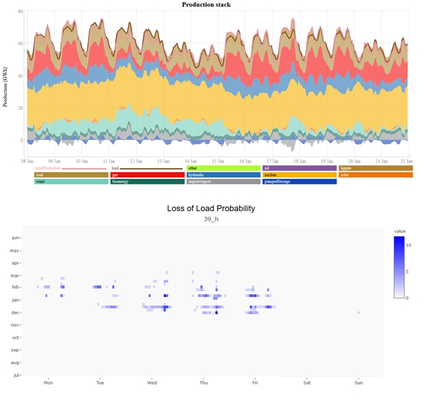
Simulation results involve all of the variables related to the system operation (unit-commitment and generation level for each unit, flow through each tie-line), hour by hour and for all Monte-Carlo years. Results such as loss of load duration, unsupplied energy or generation margins give an assessment of the security of supply in the different zones of the simulated system. In addition, the tool gives an account of the CO2 emissions, as well as an assessment of the economic performance of the whole system (various estimates such as operation costs, locational marginal prices, congestion fees, etc.).
Simulation results can be written with several time resolution (hourly to annual) and spatial resolution (one link, one area, one set of areas). Antares also gives the possibility to analyse the simulation results through probabilistic indicators (expected value averaged over all Monte-Carlo years, standard deviation, minimum and maximum, etc.) and through the detailed realisation of each variable for all the Monte-Carlo years. Filtering options in the software enables to select which output to write in a given study.
The Antares user interface allows to go through all the aforementioned results and to quickly cross-compare the results of several simulations. In addition, R packages have been designed in order to facilitate the reading, post-processing and visualisation of the simulation results. For instance, the following graph have been made with the antaresViz package, based on the results of an Antares simulation